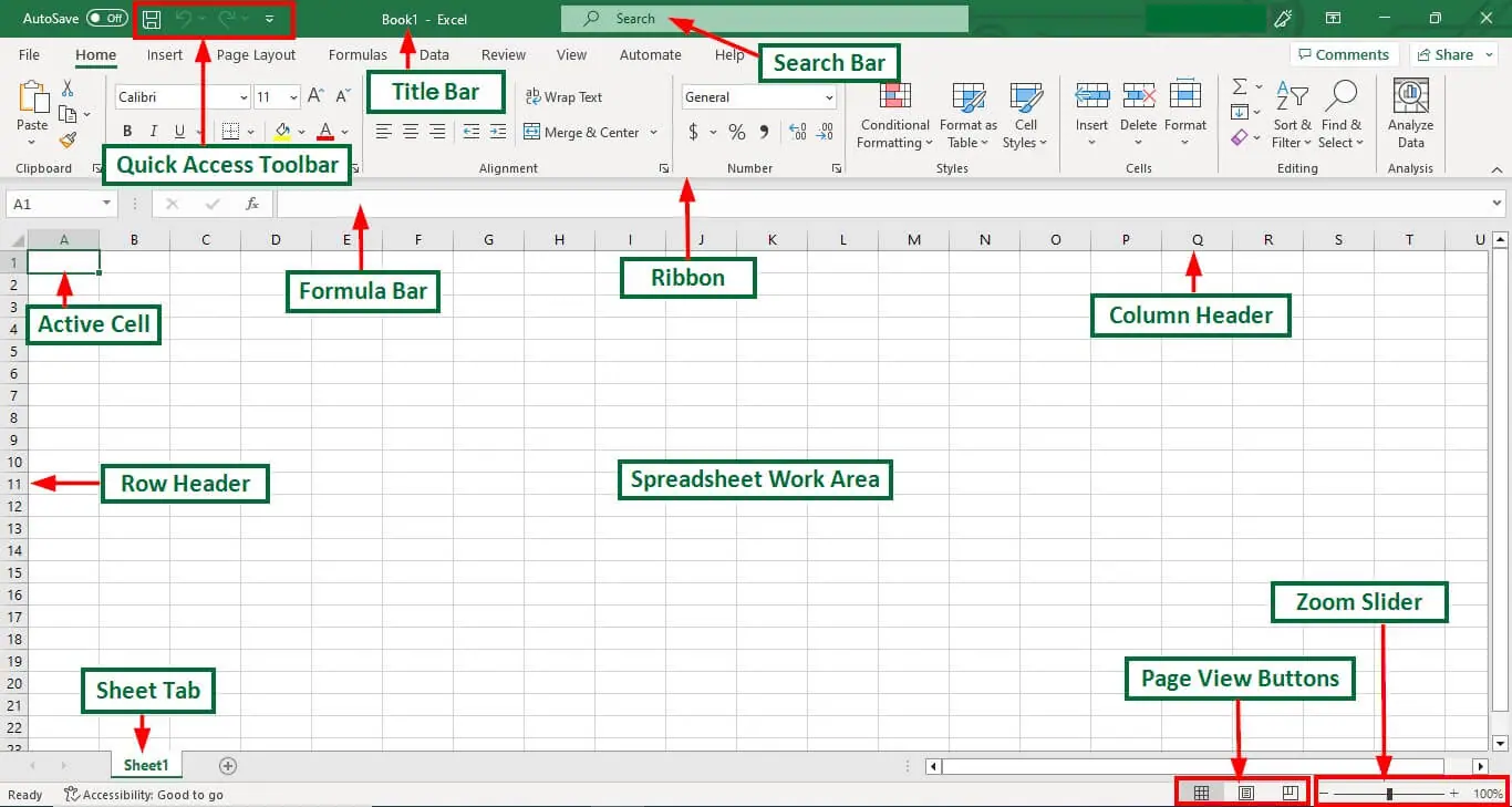
Excel is arranged in a table. Columns are identified by letters (A, B, C, etc. across the top) and rows are identified by numbers (1, 2, 3, etc., down the left side). The cell you are working in is called the active cell, is identified by the column letter and row number, in this case, cell A1. If you move down a row, you will be in cell A2. If, instead, you moved one column to the right, you will be in cell B1.
Select a row or column: A solid black arrow indicates column or row selection. To select an entire row, click on the row number, in gray, on the left. To select an entire column, click on the column letter, in gray, on the top. You will see the cells you selected are highlighted, and there is a green border around them.

Select individual cells: A thick white cross indicates cell selection. Click in the middle of a cell to select that cell. Hold down the mouse or click shift to select more cells.

Resize a column or row: A black cross with arrows on either side indicates resizing. Click on the edge of a row or column, and drag to resize.

Continue a sequence or formula: A black cross indicates formula completion. Select a cell or a group of cells using the white cross above. Then, hover over the solid green box in the bottom right corner; your cursor will become a black cross. Dragging down will continue a formula. For example, in the image below the user selected the numbers 0-5, and dragged down to add the numbers 6, 7, 8, etc. in the rows below.

More advanced tips:
The method above selects an entire row or column, including empty cells. If you only want to select the cells that contain data, click on the first cell you want to select, then use the commands Shift + spacebar to select all the data to the right of that cell in a row or Ctrl + spacebar (or Command + spacebar on a Mac) to select all the data below that cell in a column. Note: These commands will select the data until it reaches a blank cell. If you have missing data (empty cells in your spreadsheet), this option may not capture all of your data.
It is important to select the appropriate data format for the values you enter into a spreadsheet. From the Home ribbon, select Number format. You can identify different formats, such as Text, Number, Currency, or Date, and use the More Number Formats to find more options and variations. Using the appropriate data format will improve the presentation and increase the accuracy of your calculations.

You also have more options! For example, to increase the number of decimal places shown, select your data and click the Increase Decimal button. If you want to show fewer decimal places, select the data and click on the Decrease Decimal button. Note that Excel still stores the full value; you are only changing the presentation and there is no information loss with this option.

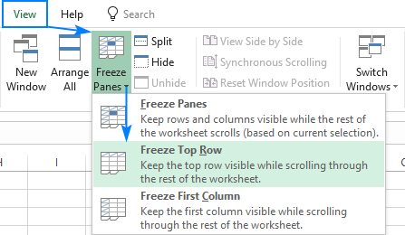
When working with large datasets in Excel, you may often want to lock certain rows or columns so that you can view their contents while scrolling to another area of the worksheet. This can be easily done by using the Freeze Panes command. If you freeze the top row, for example, you will always see the values in the top row, even if you scroll down to the bottom of a long spreadsheet.
Data validation in Excel is a feature that allows you to control the type and values of data entered into a cell or range of cells. It helps ensure data accuracy and consistency by restricting the input to a predefined set of rules. Here's how you can define data validation in Excel:


7. Save and Apply: Click "OK" to save your data validation settings.
Now, the selected cell or range will only accept data that meets the criteria you defined. If a user tries to enter data that doesn't meet the specified rules, an error message will be displayed (if configured), and the data entry will be restricted.

This feature is useful for maintaining data integrity and preventing data entry errors.
